Turn your app into a context graph
Boris Tane explains how Polylane builds and updates a context graph of an application’s infrastructure, repositories, telemetry, and resource relationships. The graph gives agents context to investigate production, assess resource health, find relevant code, and support detection and autofixes.
textBoris Tane · Oct 5, 2026 · polylane.com · Saved Nov 10, 2026
context engineering, agent infrastructure, production deployment, agent memory
We’re getting closer to self-improving software, where agents continuously read the signals your app produces and improve it automatically. To do that, an agent first has to understand how your app fits together. It needs to know which services talk to which databases, what each queue triggers, and which repository deploys what.
So, before an agent reads a single log line, it’s necessary to give it a graph of everything your app uses to run: clouds, repos, observability providers, etc.
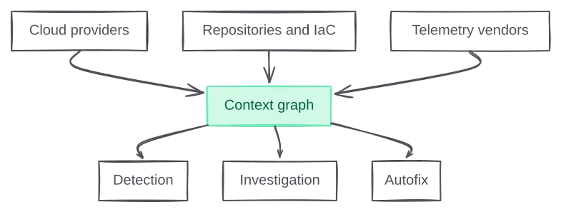
graph TB C["Cloud providers"] --> G["Context graph"] R["Repositories and IaC"] --> G T["Telemetry vendors"] --> G G --> D["Detection"] G --> I["Investigation"] G --> F["Autofix"] style G fill:#d1fae5,stroke:#6ee7b7,color:#065f46
This is the context graph. Every resource in every connected account is a node, every relationship between them is an edge, and the graph is continuously updated, as you deploy new things, delete old ones, and refactor your codebase. The context graph also encompasses all the data that lives alongside the nodes, in vector databases, in key-value stores, etc. This additional data is the difference between an agent that can traverse a graph and one that actually understands your app.
This post walks through how we turn an app into a context graph: what goes into it, how we keep it in sync with every provider, and how we connect resources across clouds without guessing.
Compute Networking Storage Databases Security Messaging Other Observability Repositories
Figure 1
Every resource in one workspace's context graph
Each dot is a resource, coloured by category.
What’s in the context graph?
The context graph is made of nodes and edges. A node is a resource: a Lambda function, a Worker, a Kubernetes deployment, a repository, a team. An edge is a typed relationship between two of them, read in one direction: a queue triggers a function, a function assumes a role and connects_to a table, a repository deploys_to the function, a team owns the repository.
Figure 2
One Lambda function and everything around it
We use Cloudflare Durable Objects for the graph itself. Each workspace on Polylane gets its own instance, with both compute and SQLite storage, so there’s no cluster to run, no connection pool to manage, and no shared tables to keep tenants apart. The graph only holds what a resource is and how it connects to other nodes.
The majority of workspaces in Polylane have fewer than 100 nodes, but a subset of customers have more than 10,000 nodes. Our solution must scale to those apps too.
under 100 56%
100 to 1,000 34%
1,000 to 10,000 9.1%
10,000 to 100,000 0.9%
Figure 3
Share of workspaces by the number of resources in their graph
One Durable Object per workspace, whatever the size.
The graph itself is two tables, nodes and edges. A node’s identity is five fields, provider, account, region, type and id, and the database derives the key from them itself, so no caller can ever build it differently:
CREATE TABLE nodes (
    provider TEXT NOT NULL,
    account TEXT NOT NULL,
    region TEXT NOT NULL,
    type TEXT NOT NULL,
    id TEXT NOT NULL,
    composite_id TEXT GENERATED ALWAYS AS ('provider#' || provider || '#account#' || account || '#region#' || region || '#type#' || type || '#id#' || id) VIRTUAL NOT NULL UNIQUE,
    data TEXT,
    created INTEGER NOT NULL,
    updated INTEGER NOT NULL,
    -- ...
);
The data field holds the properties of the node, as JSON. For a Lambda function that’s all the data returned by the AWS API when calling GetFunction. Environment variable values are stripped before anything is stored, only the keys are kept:
{
  "FunctionName": "checkout-api",
  "Runtime": "nodejs22.x",
  "Handler": "dist/index.handler",
  "MemorySize": 1024,
  "Timeout": 30,
  "Architectures": ["arm64"],
  "Role": "arn:aws:iam::123456789012:role/checkout-api-role",
  "VpcConfig": { "SubnetIds": ["subnet-0a1b2c3d"], "SecurityGroupIds": ["sg-0e4f5a6b"] },
  "EventSourceMappings": [{ "EventSourceArn": "arn:aws:sqs:eu-west-1:123456789012:orders-events", "BatchSize": 10, "State": "Enabled" }],
  "LastModified": "2026-10-04T18:22:41.000+0000",
  "RevisionId": "4c1e9a0b-7d2f-4e61-9a3c-2b8d5f0e1a77",
  "State": "Active",
  "envVarCount": 3,
  "envVarKeys": ["ORDERS_TABLE", "STRIPE_SECRET_KEY", "LOG_LEVEL"],
  "packageType": "Zip",
  "imageUri": null
}
Edges point from one node’s key to another’s, and a pair of nodes can have at most one edge of each relationship:
CREATE TABLE edges (
    source TEXT,          -- composite_id of the node the edge starts from
    target TEXT,          -- composite_id of the node it points to
    relationship TEXT,    -- connects_to, triggers, deploys_to, owns, ...
    properties TEXT,      -- JSON: the evidence the edge was drawn from
    discovered_via TEXT,  -- infrastructure_sweep, environment_variables, repository, ...
    created_by TEXT NOT NULL,
    last_edited_by TEXT NOT NULL,
    created INTEGER NOT NULL,
    updated INTEGER NOT NULL,
    UNIQUE(source, target, relationship)
);
discovered_via records how we know the relationship between the nodes. It could be through an environment variable, an integration, or manually added by a user. The properties field keeps the evidence of the connection, like the DNS record an edge was drawn from, or the image reference and what it was matched on, so an agent can check why two resources are connected.
What lives next to the graph
The context graph is not just the graph database. We also enrich each node with a wide range of additional data that the agent can access alongside it:
- A catalog that finds a resource from the name an engineer would use for it
- A resource object that remembers how each resource normally behaves, so the agent can tell healthy from broken without querying a provider
- The repository that deploys each resource, so the agent goes straight to the code that’s running on it
- Key queries, the questions worth asking about each resource when something goes wrong, prepared ahead of time
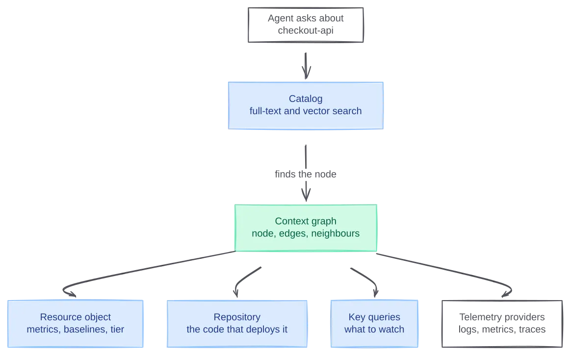
graph TB A["Agent asks about checkout-api"] --> S["Catalog<br/>full-text and vector search"] S -->|"finds the node"| G["Context graph<br/>node, edges, neighbours"] G --> R["Resource object<br/>metrics, baselines, tier"] G --> C["Repository<br/>the code that deploys it"] G --> K["Key queries<br/>what to watch"] G --> T["Telemetry providers<br/>logs, metrics, traces"] style G fill:#d1fae5,stroke:#6ee7b7,color:#065f46 style S fill:#dbeafe,stroke:#93c5fd,color:#1e3a8a style R fill:#dbeafe,stroke:#93c5fd,color:#1e3a8a style C fill:#dbeafe,stroke:#93c5fd,color:#1e3a8a style K fill:#dbeafe,stroke:#93c5fd,color:#1e3a8a
The catalog: finding the node
An agent rarely knows a node’s ID. It knows “the checkout database”. In order to use the graph and figure out its dependencies, it’s necessary to go from “the checkout database” to its ID in the cloud provider. We implemented a second Durable Object per workspace which holds a full-text search index over every node’s name and alternate names, alongside embeddings in a vector database. The agent can use this to find the ID of the database based on its human-readable name.
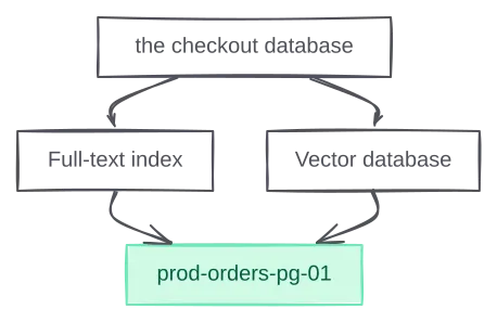
graph TB Q["the checkout database"] --> F["Full-text index"] Q --> V["Vector database"] F --> N["prod-orders-pg-01"] V --> N style N fill:#d1fae5,stroke:#6ee7b7,color:#065f46
The resource object: is it healthy?
For the workspace with thousands of cloud resources, the agent should not need to call the observability provider to know basic metrics about the resource every time it’s accessing it, it’s actually impossible given all providers have pretty stringent rate-limits.
For every resource we keep its baseline of metrics, alongside recent timeseries and common logs. This data lets an agent quickly and cheaply know if a resource is healthy or misbehaving:
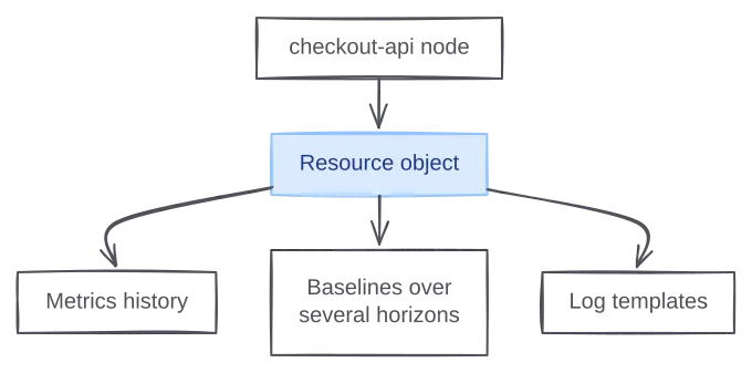
graph TB N["checkout-api node"] --> R["Resource object"] R --> M["Metrics history"] R --> B["Baselines over<br/>several horizons"] R --> L["Log templates"] style R fill:#dbeafe,stroke:#93c5fd,color:#1e3a8a
The baselines cover several horizons, so a Monday morning peak doesn’t read as an issue.
The repository: what’s running on it
An organisation can have hundreds of repositories, and an agent that has to guess which one is behind a failing service wastes its time in the wrong code. Every resource in the graph knows the repository that deploys it, and often the exact file that defines it: the Terraform module, the wrangler.toml, the task definition. When the agent needs to read code, it starts in the right place.
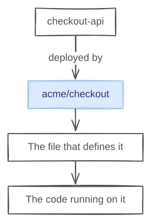
graph TB N["checkout-api"] -->|"deployed by"| R["acme/checkout"] R --> F["The file that defines it"] F --> S["The code running on it"] style R fill:#dbeafe,stroke:#93c5fd,color:#1e3a8a
Key queries: what to watch
To further improve the context we give to the agents, for each node, we compute “key queries”. Key queries are the questions an engineer would ask about every piece of their architecture when they get paged. For example, for an auth service, they will want to know:
- How many logins are failing right now, and for what reason?
- How long does token verification take at the 95th percentile?
- Is the identity provider rate limiting us?
We compute these ahead of time by looking at metrics, logs but also custom spans a developer added to their codebase, such that we can answer the type of questions impossible to answer with just metrics.
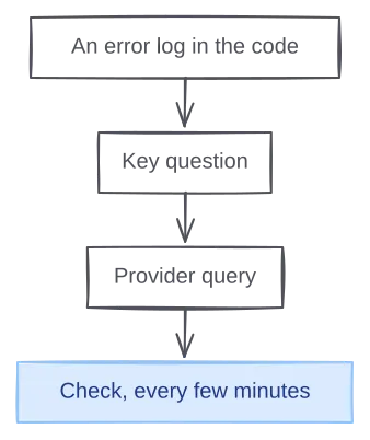
graph TB L["An error log in the code"] --> Q["Key question"] Q --> P["Provider query"] P --> C["Check, every few minutes"] style C fill:#dbeafe,stroke:#93c5fd,color:#1e3a8a
The graph is the index that joins all of this together. An agent investigating checkout-api starts from its node, walks to the database it connects to, checks that database’s baselines in its resource object, searches the repository that deploys it, and queries its logs, without ever being told where any of it lives.
How we keep the graph up to date
An app continuously evolves, and keeping the context graph in sync with the reality of the app is a complex challenge. We need to react to changes in the application and surgically create, update and delete nodes as they evolve in the application. Each cloud provider is different with different APIs and mechanisms, so we have to adapt to each:
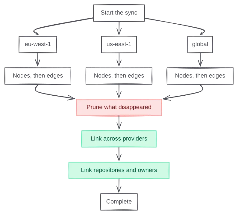
graph TB S["Start the sync"] --> RA["eu-west-1"] S --> RB["us-east-1"] S --> RC["global"] RA --> NA["Nodes, then edges"] RB --> NB["Nodes, then edges"] RC --> NC["Nodes, then edges"] NA --> P["Prune what disappeared"] NB --> P NC --> P P --> X["Link across providers"] X --> C["Link repositories and owners"] C --> D["Complete"] style P fill:#fee2e2,stroke:#fca5a5,color:#7f1d1d style X fill:#d1fae5,stroke:#6ee7b7,color:#065f46 style C fill:#d1fae5,stroke:#6ee7b7,color:#065f46
For example, for AWS we use CloudTrail, for Kubernetes we use a small Helm agent that dials out through a Cloudflare Tunnel, for Vercel we use webhooks, and for Cloudflare, we rely on audit logs.
 AWS 29%
 Kubernetes 28%
 Cloudflare 17%
 GitHub repositories 9.2%
 Railway 7.8%
 Vercel 3.7%
 Fly.io 1.7%
 Container registries 1.3%
 Convex 0.9%
 Trigger.dev 0.7%
External services 0.5%
 Supabase 0.4%
 PlanetScale 0.1%
 Render <0.1%
 Modal <0.1%
 ClickHouse Cloud <0.1%
Other 0.1%
Figure 4
Distribution of resources in customer graphs, by provider
The key constraints of syncing are how long it takes and how much of the provider’s rate limit budget it consumes. Every call a sync makes is a call the customer’s own tooling can’t, so a sync has to finish quickly and touch as little as possible. Most of them find nothing to change: a PlanetScale or Supabase sync almost never adds or removes a resource, while an AWS sync touches about 20 resources and a Kubernetes one about 12. The chart below shows how long syncs take for each provider, from the fastest tenth to the slowest, and how much each one changes.
Figure 5
How long a sync takes, and how much it changes
Completed account syncs in the last 30 days, from the sync starting to the account being marked ready. The right-hand column is every resource added or removed over the same window, divided by the number of syncs.
Connecting resources across clouds
Most applications run across multiple providers, for instance AWS for long-running containers, Cloudflare for CDN and edge-computing and Vercel for sandboxes. Syncing each cloud individually is great, but the interesting edges cross providers, because each provider only knows its own half.
After the provider work, every sync runs one shared linker over the whole workspace. A DNS record pointing at .elb.amazonaws.com connects to that load balancer, one pointing at .vercel.app to that Vercel project, .cfargotunnel.com to that tunnel. An environment variable holding an RDS endpoint connects the function to the database.
Figure 6
One request path across Cloudflare, AWS, GitHub and Datadog
The DNS record, the load balancer's listeners, the image the service runs and the Datadog metric tags each contribute some of these edges. No single provider knows the whole path.
Put together, the syncs and the linkers give every customer a graph that looks like their stack rather than like any one provider’s console.
AWS Kubernetes Cloudflare GitHub Railway Vercel
Figure 7
What's in a context graph
The twelve most common resource types, each sized and labelled by its share of those twelve. Together they make up 61% of every resource in every customer graph.
How agents use the graph
The Polylane agents get a narrow tools over the graph:
- find nodes by any field in the provider’s JSON
- read a node and its neighbours
- walk the graph in either direction, and
- compute a blast radius.
findNodes 67%
getNode 21%
getNodeEdges 7%
getInfraStats 3%
findNeighbours 1.5%
getBlastRadius 0.3%
traverseNodes <0.1%
Figure 8
Which graph tools agents call
Each tool's share of every graph tool call agents made in the last 30 days, across every customer workspace.
Agents really like findNodes as they use it to filter nodes across any dimensions. For example they can find all the AWS Lambda function with Go runtime in a single call.
| Tool | Share of calls | Median | p95 |
|---|---|---|---|
findNodes | 67% | 128 ms | 533 ms |
getNode | 21% | 519 ms | 1,494 ms |
getNodeEdges | 7.0% | 115 ms | 878 ms |
getInfraStats | 3.0% | 98 ms | 328 ms |
findNeighbours | 1.5% | 136 ms | 549 ms |
getBlastRadius | 0.3% | 118 ms | 314 ms |
traverseNodes | <0.1% | 85 ms | 259 ms |
Table 1
Graph tool latency
End to end, from the agent's tool call to its result, over the last 30 days.
The blast radius tool is used when the agent wants to know the downstream services of a specific node. It’s useful when it identifies a node as the potential cause of an incident and it wants to know grade the severity of the incident. For example, if a database fails, the services that connects_to it fail too, so the fault travels against the edge. If a queue fails, the functions it triggers stop, so the fault travels with it.
Figure 9
The blast radius of a failing database
The fault starts at orders-db (red) and travels against every connects_to edge, reaching the function and the service that use it, then the target group in front of the service (amber). The queue and the repository are connected but outside the radius.
Agents are only as good as the context you give them. We built a system to create a rich context graph for any application, and it powers everything Polylane does.